Seed Germination Calculator

The math for this calculator came about because I wondered about testing a sample of seeds to calculate the germination rate. If I plant ten and ten sprout, then naively the rate is 100%. This is the sample germination rate, but what does that tell us about the true population germination rate? Surely it's not 100%. So I worked out the math for the binomial distribution to estimate the population germination rate from a finite sample and to calculate the credible interval of that germination rate estimate. This calculator basically answers the question, "What is the resolving power of an experiment where I sow n seeds, of which k germinate? What can I say about the true germination rate?" I am a super nerd.

Check my work here. I also checked the above calculator implementation of the derived analytical formulas via numerical simulations in Python, with the following results.

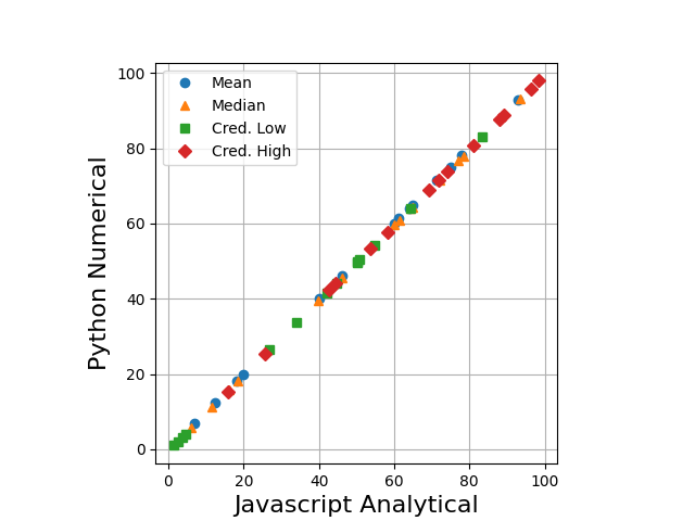
The Javascript calculator and numerical simulations show complete agreement, so I am confident in the accuracy of the calculator and underlying formulas. The Python code follows, in case you want to check my work or run the simulations yourself.

import os, sys,math
import numpy as np
import matplotlib.pyplot as plt

# calculate the mean, median, and 95% credible interval
# limits for statistics of k germinations from n total seeds
def numerical(n,k):

    # number of repetitions to run
    r = 100000

    ps = np.arange(0.01,1.0,0.01)
    ps = np.vstack((ps,ps))

    for i in range(ps.shape[1]):

        p = ps[0,i]

        sample = np.random.rand(n,r)
        q = np.less(sample,p)
        s = np.sum(q,axis=0)

        ps[1,i] = np.sum(np.equal(s,k))

    # manually include p=0 limit
    if k!=0:
        ps = np.hstack((np.expand_dims(np.array((0.0,0)),1),ps))
    else:
        ps = np.hstack((np.expand_dims(np.array((0.0,n)),1),ps))

    # manually include p=1 limit
    if k!=n:
        ps = np.hstack((ps,np.expand_dims(np.array((1.0,0)),1)))
    else:
        ps = np.hstack((ps,np.expand_dims(np.array((1.0,n)),1)))

    # normalize over konstant k
    total = np.sum(ps[1])
    ps[1]/=total

    cs = np.cumsum(ps,axis=1)
    cs = np.vstack((ps[0],cs[1]))

    mean = np.sum(np.multiply(ps[0],ps[1]))
    median = np.interp(0.5,cs[1],cs[0])
    x95lo = np.interp(0.025,cs[1],cs[0])
    x95hi = np.interp(0.975,cs[1],cs[0])

    return(mean,median,x95lo,x95hi)


# javascript analytical solution results
#  n    k       mean    median  95lo    95hi
#-------------------------------------------
ref = np.array([[30,	3,	12.5,	11.7,	3.63,	25.7],
[6,	5,	75,	77.1,	42.1,	96.3],
[13,	2,	20,	18.6,	4.65,	42.8],
[9,	1,	18.1,	16.2,	2.52,	44.4],
[19,	14,	71.4,	72.1,	50.8,	88.1],
[23,	15,	64,	64.3,	44.6,	81.2],
[39,	31,	78,	78.5,	64.3,	89.1],
[40,	38,	92.8,	93.5,	83.4,	98.4],
[42,	2,	6.81,	6.16,	1.46,	15.8],
[48,	19,	40,	39.8,	26.9,	53.7],
[63,	29,	46.1,	46.1,	34.2,	58.2],
[73,	45,	61.3,	61.4,	50.1,	71.9],
[89,	58,	64.8,	64.9,	54.7,	74.2],
[98,	59,	60,	60,	50.2,	69.3]])

results = np.copy(ref)

# run the numerical simulation
for j in range(ref.shape[0]):
    this_n = int(ref[j,0])
    this_k = int(ref[j,1])

    print('running',this_n,this_k)
    sys.stdout.flush()

    results[j,2:] = numerical(this_n,this_k)

# make everything easy to plot
f_mean = np.vstack((ref[:,2],results[:,2]))
f_median = np.vstack((ref[:,3],results[:,3]))
f_xlo = np.vstack((ref[:,4],results[:,4]))
f_xhi = np.vstack((ref[:,5],results[:,5]))

# make a comparison plot between analytical and numerical data
fig, ax = plt.subplots()
ax.plot(f_mean[0,:],100.0*f_mean[1,:],'o',label='Mean')
ax.plot(f_median[0,:],100.0*f_median[1,:],'^',label='Median')
ax.plot(f_xlo[0,:],100.0*f_xlo[1,:],'s',label='Cred. Low')
ax.plot(f_xhi[0,:],100.0*f_xhi[1,:],'D',label='Cred. High')
plt.legend(loc='upper left')
plt.xlabel('Javascript Analytical', fontsize=16)
plt.ylabel('Python Numerical', fontsize=16)
ax.grid()
plt.gca().set_aspect('equal')
fig.savefig('comparison.png')

Seed Germination Rate Estimation